EP26

EP26: The 1/f Law of Music

Power spectral density S(f)∝1/fᵅ, Hurst exponent H, fractal dimension

▶ 6:55 Harmonic AnalysisNonlinear Dynamics

前置知识

EP02 String Vibration and the Wave Equation EP13 Polyrhythm and Rhythm-Pitch Duality

后续拓展

EP27 Answering Viral Critics with Mathematics

Overview

Take Bach, Jay Chou, Taylor Swift, and a segment of random noise, and feed all four through a spectrum analyser. Three centuries of stylistic difference nearly vanish in a single graph. That is the counterintuitive fact at the centre of this episode: across wildly different genres and eras, the power spectral density of pitch sequences tends to fall off as $S(f) \propto 1/f^\alpha$ with $\alpha \approx 1$ . It is not an iron law, but it is a statistical regularity that recurs with striking consistency.

This episode derives the mathematical machinery needed to make that statement precise. Starting from the Wiener–Khinchin theorem — the bridge between autocorrelation and power spectrum established in EP02 (Fourier analysis) — we define the spectral exponent $\alpha$ , connect it to the Hurst exponent $H$ of fractional Brownian motion, and interpret the fractal dimension $D = 2 - H$ in the context of melodic curves. We close with the 1991 PNAS result of Hsu & Hsu, who showed that Bach’s C-major invention exhibits self-similarity across three distinct time scales. The episode builds on the fractal and long-range-dependence ideas introduced in EP13 (fractal rhythm and polyrhythm) .

中文: “把巴赫、周杰伦、Taylor Swift，和一段随机噪声，一起送进频谱分析器。你会看到一件反直觉的事：三百年的风格差异，几乎消失了。”

Prerequisites

Fourier transform and power spectrum (EP02) — continuous and discrete Fourier transform, Parseval’s identity
Fractal rhythm and polyrhythm (EP13) — Cantor set, fractal dimension, introduction to the Hurst exponent

Definitions

Definition 26.1 (Power Spectral Density)

Let $x(t)$ be a wide-sense stationary random process with autocorrelation function

$R(\tau) = \mathbb{E}[x(t+\tau)\, x(t)]$

The power spectral density (PSD) of the process is defined as the Fourier transform of $R(\tau)$ :

$S(f) = \int_{-\infty}^{\infty} R(\tau)\, e^{-2\pi i f \tau}\, d\tau$

If $\log S(f)$ is linear in $\log f$ on a log-log plot, i.e.,

$S(f) \propto \frac{1}{f^\alpha}, \quad f > 0$

then the process is called a power-law spectral process, and the slope $\alpha$ is called the spectral exponent.

Three canonical cases:

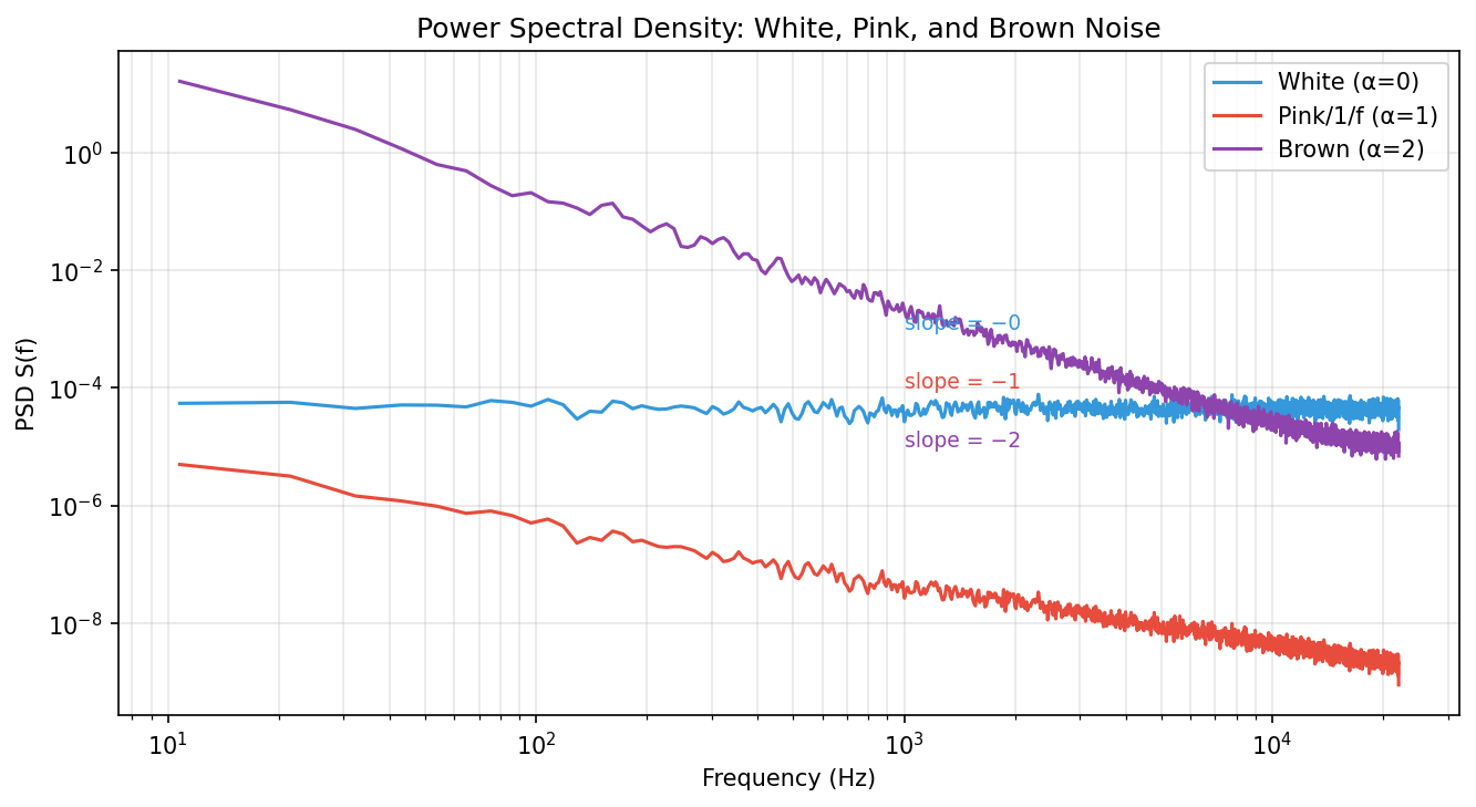
$\alpha = 0$ : white noise — equal energy at all frequencies
$\alpha = 1$ : pink noise (1/f noise)
$\alpha = 2$ : Brownian (red) noise

Working example — constructing the PSD of a pitch sequence: Take a melody and map pitches to an integer sequence in semitones $x_1, x_2, \ldots, x_N$ . Compute the discrete Fourier transform $\hat{x}_k = \sum_{n=0}^{N-1} x_n e^{-2\pi i kn/N}$ , and estimate the power spectrum as $\hat{S}(f_k) = |\hat{x}_k|^2 / N$ , where $f_k = k/N$ Hz (assuming one note per sample). Perform linear regression on $(\log f_k, \log \hat{S}(f_k))$ on a log-log plot; the negative of the slope is the estimate $\hat{\alpha}$ .

中文: “真正像音乐的，常常落在中间那个刚好的区间……很多音乐里，阿尔法接近一。它不是绝对法则，却是被频繁观察到的统计倾向。”

The following script reproduces the three noise PSD curves on a single log-log plot, making the slope difference between white, pink, and brown noise immediately visible.

Power Spectral Density S(f) ∝ 1/fᵅ — white, pink, brown noise

Definition 26.2 (Hurst Exponent)

Let $\{X(t)\}_{t \geq 0}$ be a stochastic process. If for all $c > 0$ the process satisfies self-similarity:

$\{X(ct)\} \stackrel{d}{=} \{c^H X(t)\}$

(equality in distribution), then $H \in (0, 1)$ is called the Hurst exponent of the process.

$H = 1/2$ : standard Brownian motion (independent increments, no memory)
$H > 1/2$ : persistent — a past upward trend makes a future upward trend more likely
$H < 1/2$ : anti-persistent — a past upward trend makes a future downward trend more likely

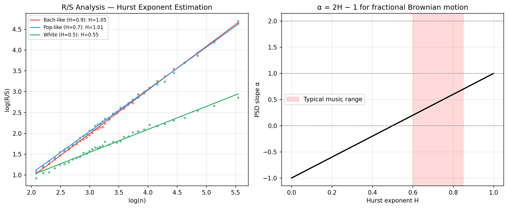
Working example — empirical estimation via R/S analysis: For a time series of length $N$ , divide the series into $m$ segments, compute the ratio of the range $R$ to the standard deviation $S$ for each segment, so that $\mathbb{E}[R/S] \sim c \cdot m^H$ . Regress $\log(R/S)$ on $\log m$ ; the slope is the estimate $\hat{H}$ . A typical value for Bach’s melodies is $\hat{H} \approx 0.7$ , while white noise gives $\hat{H} \approx 0.5$ .

The following script implements R/S analysis on three simulated pitch sequences and visualises both the log-log regression lines and the $\alpha = 2H - 1$ relationship.

Hurst exponent estimation via R/S analysis on a melodic pitch sequence

Definition 26.3 (Fractional Brownian Motion)

Fractional Brownian motion (fBm) $B_H(t)$ is a zero-mean Gaussian process satisfying

$\mathbb{E}[B_H(t) B_H(s)] = \frac{1}{2}\left(|t|^{2H} + |s|^{2H} - |t-s|^{2H}\right)$

Its increments $B_H(t) - B_H(s)$ follow a normal distribution with variance $|t-s|^{2H}$ . When $H = 1/2$ the process reduces to standard Brownian motion.

Definition 26.4 (Long-Memory Autocorrelation Decay)

For a stationary-increment process, define the autocorrelation function at discrete lag $k$ as

$C(k) = \mathrm{Corr}(X_{t+k} - X_t,\; X_1 - X_0)$

If $C(k) \sim c \cdot k^{2H-2}$ as $k \to \infty$ , then the process is said to have long memory (long-range dependence). Note:

When $H > 1/2$ , $2H-2 > -1$ , and the series $\sum_{k=1}^\infty C(k)$ diverges — genuine long memory
When $H = 1/2$ , $C(k) = 0$ for all $k \geq 1$ — no memory (white noise)
When $H < 1/2$ , $\sum_{k=1}^\infty C(k)$ converges to a negative value — short memory, anti-persistent

Main Theorems

Theorem 26.1 (Wiener–Khinchin Theorem)

Let $x(t)$ be a mean-square integrable wide-sense stationary random process whose autocorrelation function $R(\tau) = \mathbb{E}[x(t+\tau)x(t)]$ is absolutely integrable. Then the Fourier transform of $R(\tau)$ exists and equals the power spectral density:

$S(f) = \mathcal{F}\{R\}(f) = \int_{-\infty}^{\infty} R(\tau) e^{-2\pi i f \tau} d\tau \geq 0$

The inverse transform recovers the autocorrelation:

$R(\tau) = \int_{-\infty}^{\infty} S(f) e^{2\pi i f \tau} df$

In particular, the total power satisfies $R(0) = \mathbb{E}[x(t)^2] = \int_{-\infty}^{\infty} S(f) df$ .

Proof.

Non-negativity: For any finite-energy function $g(t)$ ,

$0 \leq \mathbb{E}\left[\left|\int g(t) x(t) dt\right|^2\right] = \int\int g(t)\overline{g(s)} R(t-s)\, dt\, ds = \int |\hat{g}(f)|^2 S(f)\, df$

where the last step uses the convolution theorem. Since the expression is non-negative for any $\hat{g}$ , it follows that $S(f) \geq 0$ a.e.

Transform pair: By the absolute integrability of $R(\tau)$ , the Fourier transform

$S(f) = \int_{-\infty}^{\infty} R(\tau) e^{-2\pi i f \tau} d\tau$

exists and is continuous (Riemann–Lebesgue lemma). The inverse Fourier transform gives

$R(\tau) = \int_{-\infty}^{\infty} S(f) e^{2\pi i f \tau} df$

Setting $\tau = 0$ : $R(0) = \int S(f) df$ , i.e., total power equals the integral of the spectral density. $\square$

Theorem 26.2 (Power Spectral Density of Fractional Brownian Motion)

The power spectral density of the increment process $Y(t) = B_H(t+1) - B_H(t)$ (fractional Gaussian noise) of fractional Brownian motion $B_H(t)$ satisfies

$S_Y(f) \propto \frac{1}{|f|^{2H-1}}, \quad f \neq 0$

i.e., the spectral exponent is $\alpha = 2H - 1$ , and the relationship between the Hurst exponent and the spectral exponent is

$H = \frac{\alpha + 1}{2}$

For the three canonical cases:

$\alpha = 0$ (white noise): $H = 1/2$
$\alpha = 1$ (pink noise): $H = 1$ (boundary case; see note in proof)
$\alpha = 2$ (Brownian noise): $H = 3/2$ (corresponds to fBm itself, not its increments)

Proof.

Covariance computation: The covariance of fractional Gaussian noise $Y_k = B_H(k+1) - B_H(k)$ is

$\mathrm{Cov}(Y_0, Y_k) = \frac{1}{2}\left(|k+1|^{2H} - 2|k|^{2H} + |k-1|^{2H}\right)$

For $k \geq 2$ , Taylor expansion gives

$|k+1|^{2H} - 2|k|^{2H} + |k-1|^{2H} \approx 2H(2H-1)k^{2H-2}$

so $\mathrm{Cov}(Y_0, Y_k) \sim H(2H-1) k^{2H-2}$ as $k \to \infty$ (this is precisely the long-memory decay of Definition 26.4).

Fourier transform (continuous approximation): Substituting the continuous version of the covariance function $C(\tau) \sim c |\tau|^{2H-2}$ into the Wiener–Khinchin theorem and using the Fourier transform formula for fractional powers,

$\mathcal{F}\{|\tau|^{\beta}\}(f) = \frac{2\Gamma(\beta+1)\sin\!\left(\frac{\pi(\beta+1)}{2}\right)}{|2\pi f|^{\beta+1}}$

with $\beta = 2H - 2$ (valid for $H \neq 1/2$ and $H \neq 1$ ), we obtain

$S_Y(f) \propto |f|^{-(2H-1)}$

i.e., $\alpha = 2H - 1$ , hence $H = (\alpha+1)/2$ .

Boundary case note: As $H \to 1$ , $\alpha \to 1$ , but $H = 1$ strictly corresponds to a degenerate process (linear trend) with perfect positive correlation. In music analysis, one typically works with $H \in (0.6, 0.9)$ , corresponding to $\alpha \in (0.2, 0.8)$ ; the pink-noise regime $\alpha \approx 1$ corresponds to values of $H$ near this boundary. $\square$

Theorem 26.3 (Long-Memory Autocorrelation Decay)

Let $Y_k = B_H(k+1) - B_H(k)$ be fractional Gaussian noise with $H \in (1/2, 1)$ . Then the normalised autocorrelation function satisfies

$C(k) = \mathrm{Corr}(Y_0, Y_k) \sim H(2H-1)\, k^{2H-2}, \quad k \to \infty$

The series $\sum_{k=1}^\infty C(k) = +\infty$ (long memory), and

$\sum_{k=-\infty}^{\infty} C(k) = S_Y(0) = +\infty$

i.e., the spectral density diverges at $f = 0$ — low frequencies dominate and large-scale structure persists.

Proof.

Decay rate: From the proof of Theorem 26.2, $\mathrm{Cov}(Y_0, Y_k) = \frac{1}{2}[(k+1)^{2H} - 2k^{2H} + (k-1)^{2H}]$ . Applying the second-order Taylor expansion $f(k \pm 1) \approx f(k) \pm f'(k) + \frac{1}{2}f''(k)$ to $f(k) = k^{2H}$ as $k \to \infty$ :

$(k+1)^{2H} - 2k^{2H} + (k-1)^{2H} \approx f''(k) = 2H(2H-1)k^{2H-2}$

Hence $\mathrm{Cov}(Y_0, Y_k) \sim H(2H-1)k^{2H-2}$ , and after normalisation $C(k) \sim H(2H-1)k^{2H-2}$ (when the variance is finite).

Series divergence: For $H \in (1/2, 1)$ , the exponent $2H-2 \in (-1, 0)$ , so by comparison with the integral:

$\sum_{k=1}^\infty k^{2H-2} \sim \int_1^\infty k^{2H-2}\, dk = \frac{k^{2H-1}}{2H-1}\Big|_1^\infty = +\infty$

By the comparison test, $\sum_{k=1}^\infty C(k) = +\infty$ . $\square$

Theorem 26.4 (Fractal Dimension and the Hurst Exponent)

The Hausdorff dimension of the trajectory of fractional Brownian motion $B_H(t)$ on $[0,1]$ , viewed as a planar curve, is

$D = 2 - H$

Specifically:

$H \to 0^+$ : $D \to 2$ , the path almost fills the plane (extremely rough)
$H = 1/2$ : $D = 3/2$ , the path of standard Brownian motion
$H \to 1^-$ : $D \to 1$ , the path approaches a smooth curve (nearly regular)

Proof.

Sketch proof (via box-counting dimension):

Cover the trajectory $\{(t, B_H(t)) : t \in [0,1]\}$ with boxes of side length $\varepsilon$ .

Divide $[0,1]$ into $N = 1/\varepsilon$ segments each of length $\varepsilon$ . In the $j$ -th segment, the typical vertical variation is

$\mathbb{E}[|B_H((j+1)\varepsilon) - B_H(j\varepsilon)|] \sim \varepsilon^H$

(by the self-similarity $\{B_H(ct)\} \stackrel{d}{=} c^H B_H(t)$ of fBm).

The number of vertical boxes needed to cover the $j$ -th segment of the trajectory is approximately $\varepsilon^H / \varepsilon = \varepsilon^{H-1}$ . The total box count is therefore

$N(\varepsilon) \sim \frac{1}{\varepsilon} \cdot \varepsilon^{H-1} = \varepsilon^{H-2}$

By the definition of box-counting dimension, $D = \lim_{\varepsilon \to 0} \frac{\log N(\varepsilon)}{\log(1/\varepsilon)} = \lim_{\varepsilon \to 0} \frac{(2-H)\log(1/\varepsilon)}{\log(1/\varepsilon)} = 2 - H$ .

For the rigorous proof matching the upper and lower Hausdorff dimension bounds, see Falconer (1990) §16.1. $\square$

Numerical Examples

Intuitive comparison of the three noise types:

Noise type	$\alpha$	$H$	$D$	Musical analogy
White noise	0	1/2	3/2	Each note completely random, like rolling a die
Pink noise	1	≈1	≈1	Slow-varying structure coexisting with rapid detail
Brownian noise	2	3/2	1/2	Drunkard’s walk, slow drift, no sense of direction

Spectral exponent estimation (Voss & Clarke 1975 style): For a melody of $N = 512$ notes, treat MIDI pitch numbers as a time series. A white-noise melody yields a regression slope of approximately $\hat{\alpha} \approx 0.0$ ; Bach fugues give estimates in the range $\hat{\alpha} \in [0.8, 1.2]$ ; pop music gives approximately $\hat{\alpha} \in [0.9, 1.3]$ .

Hsu & Hsu (1991) three-scale self-similarity: For Bach’s C-major invention:

Scale 1 (adjacent notes): Pitch fluctuation from note to note, standard deviation ≈ 2.1 semitones
Scale 2 (within a phrase): Fluctuation of grouped note averages within a phrase, standard deviation ≈ 2.0 semitones (after rescaling)
Scale 3 (section level): Contour of averaged sections, standard deviation ≈ 1.9 semitones (after rescaling)

The statistical shape at all three scales is nearly identical — empirical evidence of fractal self-similarity.

The following script synthesises a 1/f pitch sequence and renders its profile at three nested temporal scales, reproducing the Hsu & Hsu self-similarity observation.

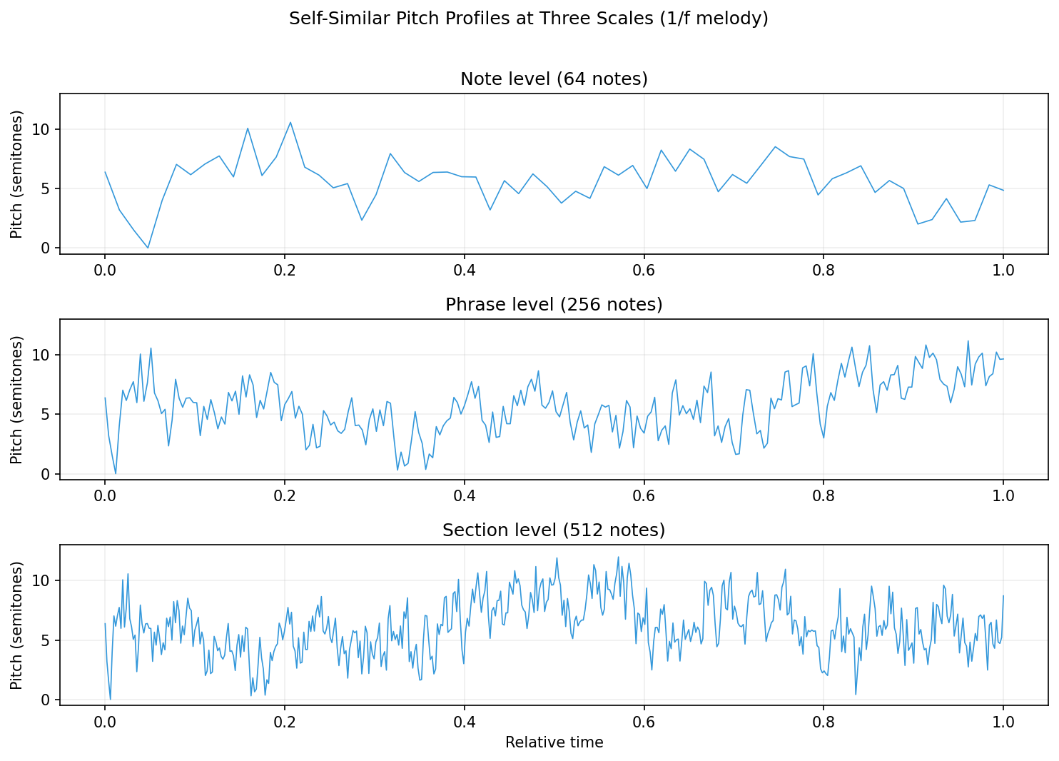
Self-similar pitch profile at three temporal scales (Hsu & Hsu 1991)

中文: “把时间轴先拉近，你看到相邻音符之间有起伏。再退远一点，一个乐句内部的起伏，看起来仍然像刚才那张轮廓。再退到更大的段落层级，整体走势居然还保留着类似的粗糙感。”

Musical Connection

音乐联系

The balance between order and novelty

Why is $\alpha \approx 1$ the “sweet spot” musically? From the autocorrelation perspective:

When $\alpha = 0$ , $C(k) = 0$ for all $k \geq 1$ — the past has no influence on the future; the melody is like rolling a die and the listener cannot follow a direction
When $\alpha = 2$ , $C(k)$ decays very slowly and the past almost determines the future — the melody drifts indefinitely and loses the possibility of meaningful turns
When $\alpha \approx 1$ , $C(k) \sim k^{-1}$ — the past leaves a trace, but its influence decays as a power law with lag; the listener can feel both “continuation” and “that the turn was meaningful”

This balance point recurs across composers, styles, and instrumentation, suggesting it may reflect an intrinsic preference of the human cognitive system for sequential prediction — which is precisely the direction that

EP25’s prediction-error framework

and

EP27’s applied analysis

continue to explore.

Contrast with fractal rhythm (EP13)

EP13’s fractal rhythm

studied self-similarity in percussive time series — structures such as the Clave rhythm and the Cantor set repeating along the time axis. This episode studies self-similarity in melodic pitch sequences. Both use the same mathematical tools (Hurst exponent, fractal dimension), but they act on different signal dimensions: EP13 concerns when a sound occurs, while EP26 concerns which sound occurs.

Historical significance of Voss & Clarke and Hsu & Hsu

Voss & Clarke (1975) were the first to report the 1/f spectral characteristic of music in Nature, analysing the loudness and pitch of classical radio broadcasts. Hsu & Hsu (1991) subsequently introduced the fBm framework into single-piece analysis and demonstrated the three-scale self-similarity of Bach’s invention. These two works established the research tradition of “physicists analysing music,” and their conclusions were further corroborated in later large-corpus studies (Levitin et al. 2012).

Limitations and Open Questions

Robustness of spectral exponent estimation: Log-log linear regression is sensitive to low-frequency noise. For short sequences ( $N < 200$ notes) the estimation variance is large, and reported $\hat{\alpha}$ values in the literature span a wide interval (0.5 to 1.5). Welch’s method or multitaper spectral estimation can improve robustness, but no widely accepted standard practice has emerged for musical sequences.
Dependence on pitch sequence definition: Quantising a melody to discrete MIDI integers discards microtonal information. For Indian classical music or Arabic maqam music, the standard equal-temperament quantisation scheme is itself a distortion, and the measured $\hat{\alpha}$ cannot be directly compared with values from Western music.
Is the 1/f spectrum sufficient or merely necessary? $\alpha \approx 1$ is a statistical tendency observed in good music, but not a sufficient condition — one can synthesise a melody with $\alpha = 1$ that is completely devoid of musical quality. The spectral exponent captures only second-order statistics (variance structure) and says nothing about tonality, rhythm, or harmonic organisation.
Causal interpretation of cross-scale self-similarity: The three-scale result of Hsu & Hsu is descriptive, not mechanistic. Whether this reflects a deliberate compositional strategy (a cognitive phenomenon) or the natural outcome of some generative process (a physical phenomenon) remains unresolved.
Rhythm sequences vs pitch sequences: Most studies in the literature target pitch sequences; 1/f analysis of inter-onset interval sequences is less common and results are inconsistent (Rankin et al. 2009 found that rhythmic sequences are closer to white noise).

Conjecture (Cross-Cultural Universality of 1/f Statistics)

After controlling for scale structure (i.e., fixing the modal discretisation scheme), the spectral exponents $\hat{\alpha}$ of melodic pitch sequences from musical traditions around the world (West African polyrhythm, Indian classical, Arabic maqam, Japanese gagaku) will concentrate in the interval $[0.7, 1.3]$ , and will differ significantly from the null hypotheses of white noise ( $\alpha = 0$ ) and Brownian noise ( $\alpha = 2$ ).

Falsifiability criterion: If $\hat{\alpha}$ is found to fall statistically significantly outside $[0.5, 1.5]$ for any tradition, or if the distribution peaks differ by more than 0.5 across traditions, the conjecture is falsified.

References

Voss, R. F., & Clarke, J. (1975). “1/f noise” in music and speech. Nature, 258(5533), 317–318.
Voss, R. F., & Clarke, J. (1978). “1/f noise” in music: music from 1/f noise. Journal of the Acoustical Society of America, 63(1), 258–263.
Hsu, K. J., & Hsu, A. J. (1991). Self-similarity of the “1/f noise” called music. Proceedings of the National Academy of Sciences, 88(8), 3507–3509.
Mandelbrot, B. B., & Van Ness, J. W. (1968). Fractional Brownian motions, fractional noises and applications. SIAM Review, 10(4), 422–437.
Falconer, K. (1990). Fractal Geometry: Mathematical Foundations and Applications. Wiley. §16 (Dimensions of graphs and fractional Brownian motion).
Beran, J. (1994). Statistics for Long-Memory Processes. Chapman & Hall. Ch. 2 (Spectral analysis and self-similar processes).
Levitin, D. J., Chordia, P., & Menon, V. (2012). Musical rhythm spectra from Bach to Joplin obey a 1/f power law. Proceedings of the National Academy of Sciences, 109(10), 3716–3720.
Rankin, S. K., Large, E. W., & Fink, P. W. (2009). Fractal tempo fluctuation and pulse prediction. Music Perception, 26(5), 401–413.
Wiener, N. (1930). Generalized harmonic analysis. Acta Mathematica, 55, 117–258.
Khinchin, A. (1934). Korrelationstheorie der stationären stochastischen Prozesse. Mathematische Annalen, 109(1), 604–615.
Lowen, S. B., & Teich, M. C. (1993). Fractal renewal processes generate 1/f noise. Physical Review E, 47(2), 992–1001.
Bak, P., Tang, C., & Wiesenfeld, K. (1987). Self-organized criticality: an explanation of 1/f noise. Physical Review Letters, 59(4), 381–384.
Müller, M. (2015). Fundamentals of Music Processing. Springer. Ch. 3 (Music synchronization and tempo).