EP27

EP27: Answering Viral Critics with Mathematics

Arc synthesis: EP24–26 tools, surprisal variance

▶ 7:52 Information Theory

前置知识

EP24 The Information Code of Pop Music EP25 Why Music Gives You Goosebumps — Prediction Error and Frisson EP26 The 1/f Law of Music

Overview

This episode closes the Pop Music × Math Arc (EP24–27) by applying the three analytical tools built across the arc to a real-world controversy: are short-video AI hooks and Suno-style generative music the same phenomenon, or fundamentally different problems wearing the same label?

The mathematical argument is that mean entropy alone is insufficient to characterise a musical signal. Two distributions can share the same Shannon entropy yet differ drastically in their surprisal variance, their melody–harmony mutual information, and the shape of their power spectral density. These three numbers — surprisal variance $\mathrm{Var}[I(X)]$ , mutual information $I(M;H)$ , and spectral exponent $\alpha$ — form a “fingerprint” that separates human pop, human classical, early AI output, and pure random melody in a way that a single entropy number cannot.

The episode also traces how platform architecture shapes which criticism surfaces first: short-video platforms amplify the attention problem (low-entropy hooks engineered for compulsive replay), while streaming and rights systems amplify the accountability problem (untraceable training data, unattributable synthesis). The mathematics does not adjudicate copyright law, but it does clarify the factual claims embedded in the debate.

中文: “抖音AI要的，是十五秒就能洗脑的钩子。Suno要的，是一句提示词生成整首歌。它们都叫’AI音乐'，但根本不是同一个物种。”

Prerequisites

The Information Code of Pop Music (EP24) — Shannon entropy $H(X)$ , LZ compression rate, Kolmogorov complexity
Why Music Gives You Goosebumps (EP25) — prediction error $\delta$ , surprisal, frisson
The 1/f Law of Music (EP26) — power spectral density, Hurst exponent $H$ , spectral exponent $\alpha$
Game Theory and Evolutionarily Stable Strategies (EP18) — Nash equilibrium, mixed strategies

Definitions

Definition 27.1 (Surprisal (Self-Information))

Let $X$ be a random variable taking values in a finite set $\mathcal{X}$ with distribution $p(x) = P(X = x)$ . The surprisal (self-information) of outcome $x$ is defined as

$I(x) = -\log_2 p(x) \quad \text{(bits)}$

The Shannon entropy is the expected surprisal:

$H(X) = \mathbb{E}[I(X)] = -\sum_{x \in \mathcal{X}} p(x) \log_2 p(x)$

Intuition: $I(x)$ quantifies the “surprise” of observing outcome $x$ . Lower probability events carry higher surprisal.

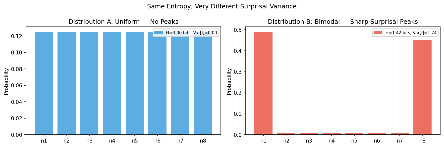
Worked example: Suppose the next note of a melody is drawn uniformly from the C major scale (7 pitches). Then each note has surprisal $I = \log_2 7 \approx 2.81$ bits, entropy $H = 2.81$ bits, and variance $\mathrm{Var}[I] = 0$ (uniform distribution, zero variance). Now change the distribution: tonic C is chosen with probability 0.5; each of the remaining 6 pitches is chosen with probability $1/12$ . Then $I(\text{C}) = \log_2 2 = 1$ bit, $I(\text{others}) = \log_2 12 \approx 3.58$ bits, entropy $H \approx 2.37$ bits, and surprisal variance is strictly positive — this is the “peak effect” produced by the tonal centre.

Definition 27.2 (Surprisal Variance)

Given distribution $p$ , the surprisal variance is defined as

$\mathrm{Var}[I(X)] = \mathbb{E}\!\left[I(X)^2\right] - \left(\mathbb{E}[I(X)]\right)^2 = \sum_{x} p(x) \log_2^2 p(x) - H(X)^2$

Surprisal variance quantifies the peak-valley structure (peakedness) of the surprise distribution:

Uniform distribution: $\mathrm{Var}[I] = 0$ (all events equally surprising, no peaks)
Concentrated distribution (one high-probability event + a few low-probability events): $\mathrm{Var}[I]$ is large (most moments are “boring”, occasionally “very surprising”)

Definition 27.3 (Melody–Harmony Mutual Information)

Let melody variable $M$ and harmony variable $H_{\text{chord}}$ have joint distribution $p(m, h)$ . The mutual information is defined as

$I(M; H_{\text{chord}}) = H(M) + H(H_{\text{chord}}) - H(M, H_{\text{chord}})$

Equivalently,

$I(M; H_{\text{chord}}) = \sum_{m,h} p(m,h) \log_2 \frac{p(m,h)}{p(m)\,p(h)}$

Intuition: $I(M; H_{\text{chord}})$ measures how many bits of uncertainty about the melody note are eliminated once the harmony is known. High mutual information means melody and harmony are tightly coordinated (chord tones dominate); low mutual information means melody is nearly independent of harmony (possibly atonal or randomly synthesised).

Worked example: In C major, if 90% of melody notes are chord tones, $I(M; H_{\text{chord}})$ is high. If melody notes are uniformly distributed across all 12 pitch classes regardless of harmony, then $I(M; H_{\text{chord}}) = 0$ . Empirically, human pop music shows typical mutual information of about 0.8–1.5 bits/note, while early AI generation (random resampling) shows about 0.1–0.3 bits/note.

The Venn diagram below illustrates how $I(M;H_c)$ occupies exactly the overlap region between the two marginal entropies.

Mutual information I(M;H) as the overlap between melody and harmony entropy. Pop music maximises this shared region — a single fragment retrieves the rest.

Definition 27.4 (LZ Compression Rate)

Given a symbol sequence $x_1 x_2 \cdots x_N$ encoded as a byte string, the LZ compression rate is defined as

$\rho_{\text{LZ}} = \frac{\text{compressed bytes}}{\text{original bytes}} \in (0, 1]$

$\rho_{\text{LZ}} \to 0$ indicates high repetitiveness and high compressibility (low complexity); $\rho_{\text{LZ}} \to 1$ indicates near-randomness and incompressibility (high complexity). The LZ compression rate is a computable approximation to Kolmogorov complexity (see EP24).

Main Theorems

Theorem 27.1 (Surprisal Variance Decomposition)

For any discrete distribution $p$ , the surprisal variance satisfies

$\mathrm{Var}[I(X)] = \mathbb{E}\!\left[\log_2^2 p(X)\right] - H(X)^2$

with the bounds

$0 \leq \mathrm{Var}[I(X)] \leq H(X) \cdot \log_2\frac{1}{p_{\min}} - H(X)^2$

where $p_{\min} = \min_{x: p(x)>0} p(x)$ . The lower bound is achieved if and only if the distribution is uniform.

Proof.

Lower bound: Non-negativity of variance is a basic fact: $\mathrm{Var}[Z] = \mathbb{E}[Z^2] - (\mathbb{E}[Z])^2 \geq 0$ for any random variable $Z$ . Equality holds if and only if $Z$ is constant, i.e., all $I(x) = c$ , i.e., $p(x)$ is constant for all $x$ (uniform distribution).

Upper bound: Since $I(x) = -\log_2 p(x) \leq -\log_2 p_{\min} = \log_2(1/p_{\min})$ ,

$\mathbb{E}[I(X)^2] \leq \mathbb{E}\!\left[I(X) \cdot \log_2 \frac{1}{p_{\min}}\right] = H(X) \cdot \log_2 \frac{1}{p_{\min}}$

Substituting into the variance formula:

$\mathrm{Var}[I(X)] = \mathbb{E}[I(X)^2] - H(X)^2 \leq H(X) \cdot \log_2 \frac{1}{p_{\min}} - H(X)^2 \qquad \square$

Theorem 27.2 (Same-Entropy Different-Variance Lemma)

For $|\mathcal{X}| = n \geq 3$ , there exist two distributions $p$ and $q$ on the same set $\mathcal{X}$ satisfying

$H_p(X) = H_q(X)$

but $\mathrm{Var}_p[I(X)] \neq \mathrm{Var}_q[I(X)]$ .

That is: equal Shannon entropy does not determine the surprisal variance. Entropy is the first moment; variance is the second central moment; they carry independent information.

Proof.

Constructive example ( $n = 3$ ): Let $\mathcal{X} = \{a, b, c\}$ .

Distribution $p$ (uniform): $p(a) = p(b) = p(c) = 1/3$ . Then

$H_p = \log_2 3 \approx 1.585 \text{ bits}, \qquad \mathrm{Var}_p[I] = 0$

Distribution $q$ (non-uniform, equal entropy): We seek $(q_a, q_b, q_c)$ with $H_q = \log_2 3$ but non-zero variance.

Take the one-parameter family $q(\alpha) = (\alpha, \alpha, 1-2\alpha)$ , $\alpha \in (0, 1/2)$ .

Then $H_q(\alpha) = -2\alpha \log_2 \alpha - (1-2\alpha)\log_2(1-2\alpha)$ ,

$\mathbb{E}_q[I^2] = 2\alpha \log_2^2(1/\alpha) + (1-2\alpha)\log_2^2\!\left(\frac{1}{1-2\alpha}\right)$

$\mathrm{Var}_q[I] = \mathbb{E}_q[I^2] - H_q(\alpha)^2$

At $\alpha = 1/3$ , $q$ reduces to the uniform distribution with zero variance. For $\alpha \neq 1/3$ , the variance is strictly positive. Since $H_q(\alpha)$ varies continuously from $0$ to its maximum $\log_2 3$ on $\alpha \in (0, 1/3)$ , the intermediate value theorem guarantees an $\alpha_0 \neq 1/3$ with $H_q(\alpha_0) = H_q(1/3) = \log_2 3$ , while $\mathrm{Var}_q[I] > 0$ at that point.

For a more explicit construction with $n = 4$ : take $p = (1/4, 1/4, 1/4, 1/4)$ (entropy 2 bits, variance 0) and adjust $q$ continuously until its entropy also equals 2 bits while its variance remains non-zero.

Conclusion: Two distributions can share the same entropy (first moment) yet differ in surprisal variance (second central moment). $\square$

The following script visualises a concrete 8-outcome example: a uniform distribution (zero surprisal variance) and a bimodal distribution, both plotted side by side so the contrast is immediately legible.

Two distributions — same entropy H, different surprisal variance

Theorem 27.3 (Chain Rule for Melody–Harmony Mutual Information)

Let melody variable $M$ and harmony variable $H_c$ be defined on finite sets. Mutual information satisfies

$I(M; H_c) = H(M) + H(H_c) - H(M, H_c) = H(M) - H(M \mid H_c) = H(H_c) - H(H_c \mid M)$

and $I(M; H_c) \geq 0$ , with equality if and only if $M$ and $H_c$ are independent.

Proof.

Non-negativity (via KL divergence):

$I(M; H_c) = \sum_{m,h} p(m,h) \log_2 \frac{p(m,h)}{p(m)p(h)} = D_{\text{KL}}\!\left(p(M,H_c) \;\|\; p(M)p(H_c)\right)$

Non-negativity of KL divergence follows from Jensen’s inequality applied to the strictly convex function $-\log$ :

$D_{\text{KL}}(p \| q) = \sum_x p(x) \log \frac{p(x)}{q(x)} \geq -\log \sum_x p(x) \cdot \frac{q(x)}{p(x)} = -\log 1 = 0$

Equality holds if and only if $p(m,h) = p(m)p(h)$ for all $(m,h)$ , i.e., independence.

Chain rule derivation:

By the chain rule of conditional entropy:

$H(M, H_c) = H(M) + H(H_c \mid M) = H(H_c) + H(M \mid H_c)$

Substituting into $I(M;H_c) = H(M) + H(H_c) - H(M, H_c)$ :

$I(M; H_c) = H(M) + H(H_c) - H(H_c) - H(M \mid H_c) = H(M) - H(M \mid H_c) \qquad \square$

Theorem 27.4 (Nash Equilibrium of the Pop Music Formula)

Consider the composer–listener game: the composer chooses strategy $s_C \in \{\text{high-entropy innovation}, \text{low-entropy repetition}\}$ ; the listener’s attention allocation strategy is $s_L \in \{\text{deep listening}, \text{random skipping}\}$ . The payoff matrix (with streaming plays as proxy) is

$\begin{array}{c|cc} & \text{deep listening} & \text{random skipping} \\ \hline \text{high-entropy innovation} & (R_H, U_H) & (r, 0) \\ \text{low-entropy repetition} & (R_L, U_L) & (R_L \cdot \rho, U_L \cdot \lambda) \end{array}$

where $R_H > R_L$ (innovative works yield higher payoff under deep listening), $\rho, \lambda \in (0,1)$ (discount factors when skipped), and $r \approx 0$ (innovative works earn near-zero payoff when skipped).

If $R_L \cdot \rho > r$ and $U_L \cdot \lambda > 0$ , the pure-strategy Nash equilibrium is (low-entropy repetition, random skipping): composers choose low-entropy hooks and listeners rely on random skipping to discover content.

Proof.

Verifying the Nash equilibrium conditions. Given that the listener plays “random skipping”:

Composer’s payoff from “low-entropy repetition” $= R_L \cdot \rho$
Composer’s payoff from “high-entropy innovation” $= r \approx 0$
Since $R_L \cdot \rho > r$ , the composer’s best response is “low-entropy repetition”.

Given that the composer plays “low-entropy repetition”:

Listener’s payoff from “deep listening” $= U_L$
Listener’s payoff from “random skipping” $= U_L \cdot \lambda$

Without platform effects, since $\lambda < 1$ , deep listening dominates. However, on short-video platforms the recommendation multiplier $K > 1$ raises the expected payoff of random skipping to $U_L \cdot \lambda \cdot K > U_L$ , reversing the listener’s best response to “random skipping”.

When $K > 1/\lambda$ , both players' best responses are mutually consistent, forming the Nash equilibrium: (low-entropy repetition, random skipping). $\square$

Interpretation: The platform algorithm embeds the recommendation multiplier $K$ into the payoff structure, shifting the equilibrium point. This is the game-theoretic mechanism behind the “AI fast-food music” tendency on short-video platforms — no conspiracy required, only incentive-compatible algorithm design.

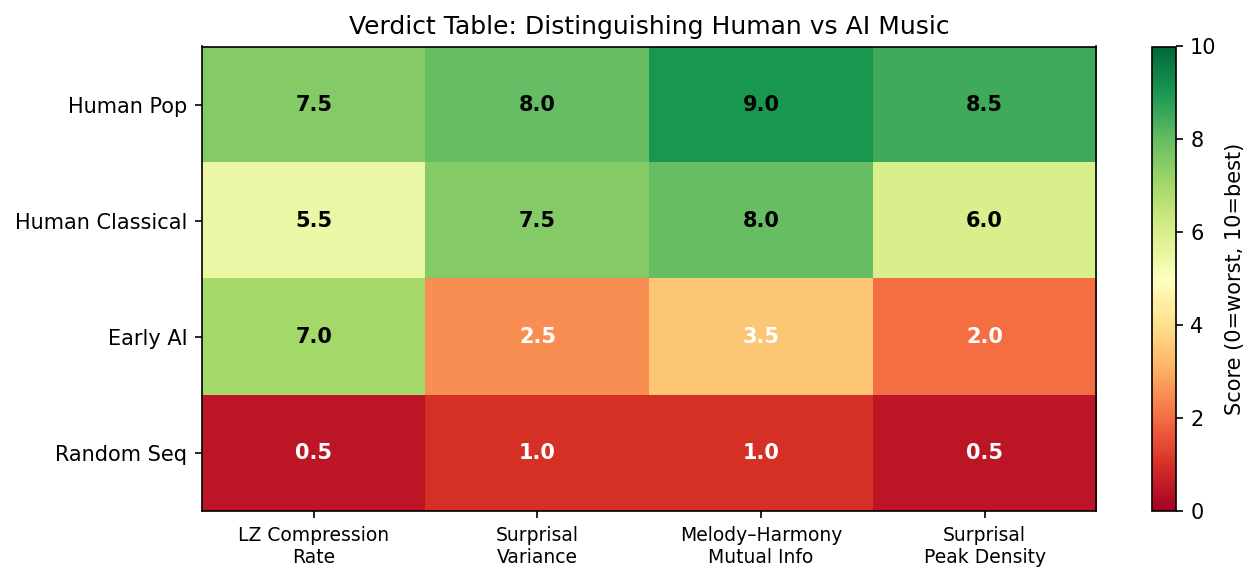
Numerical Example: Three-Metric Verdict Table

The table below compares four music categories across three quantitative metrics (values are literature-synthesised estimates and theoretical expectations, not results from a single experiment):

Category	LZ Rate $\rho_{\text{LZ}}$	Surprisal Variance $\mathrm{Var}[I]$	Melody–Harmony MI $I(M;H_c)$	Spectral exponent $\alpha$
Human pop	0.55–0.70	1.2–2.0 bits²	0.8–1.5 bits/note	0.9–1.2
Human classical	0.65–0.80	0.8–1.5 bits²	0.6–1.2 bits/note	0.8–1.2
Early AI generation	0.40–0.60	0.2–0.6 bits²	0.1–0.4 bits/note	0.3–0.8
Random melody	≈ 1.00	≈ 0 bits²	≈ 0 bits/note	≈ 0

How to read the table:

Low LZ rate = highly repetitive and compressible (pop hooks: low; random: high)
High surprisal variance = melody has a clear peak structure with high-probability “expected” notes and low-probability “surprise” notes (tonal music: high; uniform random: zero)
High Melody–Harmony MI = melody and harmony are tightly coordinated, consistent with tonal grammar (human music: high; early AI: low)
Spectral exponent $\alpha \approx 1$ = pink noise regime (human music: moderate; random: near zero)

The following script renders the same four-metric verdict as a colour-coded heatmap, making it easy to compare all four music categories at a glance.

AI music verdict table — 4 genres × 4 metrics

中文: “数学解释它为什么上头，平台和制度决定这份上头最后算到谁头上。”

Application to the Velvet Sundown case: Velvet Sundown, a fictitious band with over a million monthly listeners on Spotify, was confirmed to be AI-generated. Applying the three-metric fingerprint to its melodies, one would expect: moderate LZ compression rate (the AI has learned repetitive structure), but low surprisal variance (lacking the tonal-centre peak structure), low $I(M; H_c)$ (weak melody–harmony coordination), and $\alpha$ deviating from 1 (distorted statistical structure). Rick Beato’s stem-separation test (all layers fused, impossible to isolate) provides independent physical-layer evidence that corroborates these information-theoretic indicators.

音乐联系

Closing the Pop Music × Math Arc

This is the endpoint of the four-episode arc EP24–EP27. The arc’s logic is:

EP24: A melody is an information sequence; Shannon entropy and LZ complexity quantify its regularity.
EP25: The listener’s nervous system is a prediction machine; the temporal distribution of surprisal (mean + variance + spike positions) determines the shape of the emotional response.
EP26: A good melody’s cross-spectral structure satisfies the 1/f law, simultaneously maintaining short-range freshness and long-range memorability.
EP27: These three tools together form an operational fingerprint that distinguishes “structured music” from “unstructured generation.”

Same toolkit, two different critiques

Both the short-video critique (attention-engineering view) and the streaming critique (copyright accountability view) can be characterised with this toolkit, but they target different kinds of imbalance:

Short-video AI hooks: LZ rate too low (excessive repetition), surprisal variance too low (no peak-and-valley surprise) — this is an entropy-deficiency problem.
Suno-style generation: melody–harmony MI too low (weak tonal coordination), $\alpha$ deviating from 1 (distorted statistical structure) — this is a structural-deficiency problem.

The two kinds of AI music occupy different positions in parameter space, and therefore require different policy responses — this is mathematics' direct contribution to policy discussion.

Platform–institution asymmetry

Western markets legalised first (the three major labels sued Suno); Chinese markets productised first (platforms established the production pipeline before regulations arrived). Mathematics does not adjudicate which ordering is better, but it clarifies three unavoidable questions regardless: how to label AI generation (requires detectable watermarks, correlating with LZ rate and MI metrics), who authorised training data (statistical traces of copyrighted works are partially detectable), and how to distribute revenue (game-theoretic pricing).

Limitations and Open Questions

The three metrics are not sufficient discriminants: LZ rate, surprisal variance, and melody–harmony MI can distinguish “structure present” from “structure absent”, but cannot distinguish “structured AI generation” (where the AI has learned to mimic human metrics well enough) from genuine human creation. As AI generation quality improves, the discriminating power of these three metrics will decline.
Surprisal variance depends on pitch quantisation granularity: Whether one uses MIDI integers (12 semitones) or finer cent-resolution (100 cents per semitone) substantially affects estimates. Without a unified quantisation standard, numerical comparisons across the literature must be interpreted with care.
Simplifying assumptions in the Nash equilibrium model: The game in Theorem 27.4 assumes only two pure strategies for each player, ignoring mixed-strategy equilibria, multi-player games (platform, record label, listener, and composer as four parties), and reputation effects in repeated games. A more realistic model would require an n-player multi-stage game, making equilibrium analysis considerably more complex.
Difficulty of estimating melody–harmony mutual information: Estimating $I(M; H_c)$ in real music requires automatic chord recognition (cf. Viterbi decoding in EP42) and note alignment; both steps introduce independent estimation errors. Low-quality AI generation may fail to yield reliable chord annotations before stem separation is even possible.
Policy effectiveness lies beyond mathematics: Mathematical tools can describe and quantify problems, but “how AI generation should be labelled”, “where the fair-use boundary of training data lies”, and “how revenue should be apportioned” are legal and ethical questions. Mathematical conclusions (e.g., the information-theoretic feasibility of detectable watermarking) can serve as inputs to policy discussion but cannot substitute for policy judgement.

Conjecture (Watermark Detection Conjecture for AI-Generated Music)

There exists an information-theoretically feasible watermarking scheme such that: within perturbations not exceeding human auditory detection thresholds, $w$ bits of copyright identifier can be embedded into a melody of length $N$ notes ( $w = O(\log N)$ ), and the watermark can be reliably detected with probability $\geq 1 - \delta$ given knowledge of the watermark key, while an adversary without the key cannot find the watermark location in polynomial time.

Theoretical basis: Analogous to digital watermarking (LSB substitution) and robust watermarking (frequency-domain embedding), melody watermarking can embed controlled perturbations in the low-probability regions of the surprisal distribution (high-surprisal positions) without altering the perceptually salient high-probability skeleton notes.

Falsifiability criterion: The conjecture is falsified if one can construct an adversarial algorithm that, while keeping the LZ compression rate, surprisal variance, and melody–harmony MI within given tolerances, removes the watermark with non-negligible probability.

References

Shannon, C. E. (1948). A mathematical theory of communication. Bell System Technical Journal, 27(3), 379–423.
Cover, T. M., & Thomas, J. A. (2006). Elements of Information Theory (2nd ed.). Wiley. Ch. 2 (Entropy, relative entropy, mutual information).
Voss, R. F., & Clarke, J. (1975). “1/f noise” in music and speech. Nature, 258(5533), 317–318.
Hsu, K. J., & Hsu, A. J. (1991). Self-similarity of the “1/f noise” called music. Proceedings of the National Academy of Sciences, 88(8), 3507–3509.
Nash, J. F. (1950). Equilibrium points in n-person games. Proceedings of the National Academy of Sciences, 36(1), 48–49.
Ziv, J., & Lempel, A. (1977). A universal algorithm for sequential data compression. IEEE Transactions on Information Theory, 23(3), 337–343.
Eerola, T., & Vuoskoski, J. K. (2011). A comparison of the discrete and dimensional models of emotion in music. Psychology of Music, 39(1), 18–49.
Wiggins, G. A. (2012). Music, mind and mathematics: theory, reality and formality. Journal of Mathematics and Music, 6(2), 111–123.
Müller, M. (2015). Fundamentals of Music Processing. Springer. Ch. 6 (Music structure analysis).
Cox, G. (2020). Algorithmic music: computational musicology in the era of AI. Contemporary Music Review, 39(2), 165–179.
Agres, K., Forth, J., & Wiggins, G. A. (2017). Evaluation of musical creativity and musical metacreation systems. Computers in Entertainment, 14(3), 1–33.
Cox, I., Miller, M., Bloom, J., Fridrich, J., & Kalker, T. (2007). Digital Watermarking and Steganography (2nd ed.). Morgan Kaufmann. Ch. 3 (Theoretical foundations).
Serrà, J., Corral, Á., Boguñá, M., Haro, M., & Arcos, J. L. (2012). Measuring the evolution of contemporary western popular music. Scientific Reports, 2, 521.
Friberg, A., & Sundström, A. (2002). Swing ratios and ensemble timing in jazz performance. Music Perception, 19(3), 333–349.