EP31

EP31: The Warmth of Moog Has an Equation

4-pole cascade H(s), Barkhausen criterion, tanh → odd harmonics

▶ 5:58 Signal Processing

前置知识

EP09 Combination Tones and Nonlinear Acoustics

后续拓展

EP32 Chebyshev Waveshaping — Buchla and West Coast Synthesis EP19 Vibrato as FM Synthesis

Overview

Analog synthesizers and digital synthesizers sound “just different” — this perception is so widespread that it has spawned an entire mythology of “analog warmth.” But “warmth” is not mysticism: it is a concrete spectral fingerprint, composed of a specific distribution of odd harmonics, and the physical mechanism that produces this distribution is the odd-function property of the hyperbolic tangent $\tanh(x)$ .

Bob Moog’s 1965 patent filter contains two mathematical cores: four cascaded RC low-pass stages, giving a steep −24 dB/octave cutoff; and a feedback path from output to input, which creates resonance as the Barkhausen criterion ( $k = 4$ ) is approached, reaching a critical point where the entire filter self-oscillates as a sinusoidal oscillator. These two mechanisms, combined with the soft clipping nonlinearity of transistors (tanh soft limiting), together constitute the so-called “Moog sound.”

This episode derives the four-pole transfer function, the Barkhausen criterion, the tanh expansion, the odd harmonics theorem, and Zero-Delay Feedback (ZDF) numerical iteration one by one, giving the complete mathematical picture of “analog warmth.”

中文: “你有没有注意到，模拟合成器和数字合成器听起来就是不一样？那种’温暖'、‘肥厚’、‘模拟感’，到底是什么？答案藏在一个非线性函数里：tanh of x。”

Prerequisites

Nonlinear Harmonics and Combination Tones (EP09) — physical intuition for how nonlinear systems generate harmonics; the spectral components of combination tones share the same physical mechanism as tanh expansion producing odd harmonics
Vibration and Self-Oscillation (EP19) — oscillation background for the Barkhausen criterion; conditions for a sinusoidal oscillator to start

Definitions

Definition 31.1 (Single-Pole RC Low-Pass Transfer Function)

A first-order low-pass filter composed of a resistor $R$ and capacitor $C$ has the following transfer function at complex frequency $s = \sigma + i\omega$ :

$H_1(s) = \frac{1}{1 + s/\omega_c}$

where $\omega_c = 1/(RC)$ is the cutoff angular frequency. At real frequency $s = i\omega$ , the magnitude response is

$|H_1(i\omega)| = \frac{1}{\sqrt{1 + (\omega/\omega_c)^2}}$

Example: If $R = 10\,\text{k}\Omega$ and $C = 10\,\text{nF}$ , then $\omega_c = 10^4 \text{ rad/s}$ , giving a cutoff frequency of approximately 1.6 kHz.

Definition 31.2 (Moog Four-Pole Ladder Filter)

The Moog ladder filter consists of four identical first-order low-pass stages connected in series (cascade). Its open-loop transfer function is

$H(s) = \left(\frac{1}{1 + s/\omega_c}\right)^4 = \frac{\omega_c^4}{(s + \omega_c)^4}$

Adding a feedback coefficient $k$ (the output signal is inverted and multiplied by $k$ before being fed back to the input), the closed-loop transfer function is

$H_{\text{cl}}(s) = \frac{H(s)}{1 + k \cdot H(s)}$

The parameter $k \in [0, 4)$ controls resonance strength; $k = 0$ gives a pure low-pass response, while $k \to 4$ produces a strong resonance peak near the cutoff frequency.

Example (synthesizer panel correspondence): The cutoff frequency knob controls $\omega_c$ (frequency sweep), and the resonance knob controls $k$ (range 0–4).

The following block diagram illustrates the four-stage cascade structure and feedback path of the Moog ladder filter:

y(t)

−k (resonance)k = 4 → self-oscillation (Barkhausen)

Moog 4-pole ladder filter: four RC stages (each with tanh nonlinearity) plus a negative feedback path with coefficient k. At k = 4, the Barkhausen criterion is met and the filter self-oscillates.

Definition 31.3 (Hyperbolic Tangent Function and Taylor Expansion)

The hyperbolic tangent function is defined as

$\tanh(x) = \frac{e^x - e^{-x}}{e^x + e^{-x}}$

Its Taylor expansion at $x = 0$ is

$\tanh(x) = x - \frac{x^3}{3} + \frac{2x^5}{15} - \frac{17x^7}{315} + O(x^9)$

Key property: The expansion contains only odd-degree power terms ( $x, x^3, x^5, x^7, \ldots$ ), with no even-degree terms whatsoever.

Why only odd terms? $\tanh$ is an odd function: $\tanh(-x) = -\tanh(x)$ . The coefficients of even-degree terms in the Taylor expansion of an odd function must be zero (see Theorem 31.2).

Example (soft clipping behavior): $\tanh(1) \approx 0.762$ , $\tanh(2) \approx 0.964$ , $\tanh(3) \approx 0.995$ . As the input grows, the output approaches ±1, producing a “soft clipping” effect.

Definition 31.4 (Warmth Coefficient)

For a nonlinear device driven by a sinusoidal input $x(t) = A\sin(\omega_0 t)$ that produces harmonics, suppose the Fourier decomposition of its output is $y(t) = \sum_{k=1}^{\infty} c_k \sin(k\omega_0 t + \phi_k)$ . The warmth coefficient is defined as

$W = \frac{\sum_{k \text{ odd}} |c_k|^2}{\sum_{k=1}^{\infty} |c_k|^2}$

that is, the fraction of total harmonic power carried by odd harmonics. $W = 1$ means the output consists entirely of odd harmonics (pure odd-function nonlinearity); $W = 0.5$ means odd and even harmonic power are equal.

Reference values:

Device type	Typical $W$
Moog ladder filter (tanh-driven)	≈ 0.95
Transistor push-pull amplifier	≈ 0.95
Vacuum tube amplifier (triode)	≈ 0.65
Single-ended transistor amplifier (asymmetric)	≈ 0.45

Definition 31.5 (Zero-Delay Feedback (ZDF))

In digital implementations, the feedback path of the Moog filter introduces a one-sample delay (digital systems are causal): the output $y[n]$ is not available at computation time $n$ , so traditional implementations substitute $y[n-1]$ , introducing cutoff frequency error and resonance frequency shift.

The Zero-Delay Feedback (ZDF) method expresses $y[n]$ as an implicit equation in itself, then solves it numerically:

$y[n] = F(x[n],\, y[n],\, y[n-1],\, \ldots)$

Newton-Raphson iteration starting from initial guess $y^{(0)} = y[n-1]$ performs each step as

$y^{(k+1)} = y^{(k)} - \frac{f(y^{(k)})}{f'(y^{(k)})}$

where $f(y) = y - F(x[n],\, y,\, \ldots)$ . Typically 3–5 iterations reach machine precision.

Main Theorems

Theorem 31.1 (High-Frequency Roll-Off of the Four-Pole Ladder Filter (−24 dB/octave))

The open-loop transfer function of the Moog four-pole ladder filter is $H(s) = \bigl(1 + s/\omega_c\bigr)^{-4}$ .

High-frequency magnitude asymptote: When $\omega \gg \omega_c$ ,

$|H(i\omega)| \approx \left(\frac{\omega_c}{\omega}\right)^4$

Roll-off slope: Every time the frequency doubles (i.e., $\omega \to 2\omega$ ), the magnitude attenuates by a factor of $1/16$ , equal to $-20\log_{10}(16) \approx -24.1$ dB.

Proof.

At $s = i\omega$ , the magnitude of the four-pole transfer function is

$|H(i\omega)| = \left|\frac{1}{1 + i\omega/\omega_c}\right|^4 = \frac{1}{\left(1 + (\omega/\omega_c)^2\right)^2}$

When $\omega \gg \omega_c$ , we have $1 + (\omega/\omega_c)^2 \approx (\omega/\omega_c)^2$ , so

$|H(i\omega)| \approx \frac{1}{(\omega/\omega_c)^4} = \left(\frac{\omega_c}{\omega}\right)^4$

Roll-off slope: Multiplying frequency by 2:

$|H(i \cdot 2\omega)| \approx \left(\frac{\omega_c}{2\omega}\right)^4 = \frac{1}{16}\left(\frac{\omega_c}{\omega}\right)^4 = \frac{1}{16}|H(i\omega)|$

The magnitude attenuates by $1/16$ , which in decibels is

$20\log_{10}\!\left(\frac{1}{16}\right) = -20\log_{10}(16) = -20 \times 1.204 = -24.08 \text{ dB}$

That is, approximately −24 dB per octave. By comparison, a single pole ( $N=1$ ) gives −6 dB/oct, two poles ( $N=2$ ) give −12 dB/oct; the four-pole configuration is the steepest common ladder topology. $\square$

Intuition: Four poles ( $s = -\omega_c$ , a fourfold root) give a fourth-power attenuation; each pole contributes −6 dB/oct, and the four add up to −24 dB/oct.

The following script plots the Bode diagram of the Moog closed-loop transfer function for different resonance coefficients k, showing the evolution from flat low-pass to resonance peak to the edge of self-oscillation.

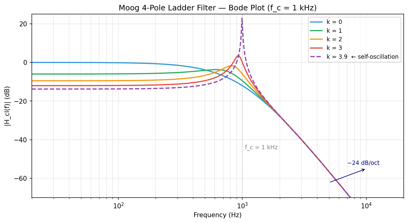
Moog 4-pole ladder filter — Bode plot with resonance k = 0, 1, 2, 3, 3.9

Theorem 31.2 (Barkhausen Criterion: The Self-Oscillation Threshold of the Moog Filter)

The Moog four-pole ladder filter (open-loop transfer function $H(s) = (1 + s/\omega_c)^{-4}$ , feedback coefficient $k$ ) exactly satisfies the Barkhausen criterion at feedback coefficient

$k = 4$

At this value there exists a real frequency $\omega^* = \omega_c$ such that

$\angle H(i\omega^*) = -\pi \quad \text{and} \quad k \cdot |H(i\omega^*)| = 1$

The closed-loop system then undergoes marginal oscillation at a frequency equal to the cutoff frequency $\omega_c$ .

Proof.

Step 1: Find the phase condition.

The phase of the single-pole $H_1(i\omega) = (1 + i\omega/\omega_c)^{-1}$ is

$\angle H_1(i\omega) = -\arctan\!\left(\frac{\omega}{\omega_c}\right)$

The total phase of the four-pole filter is

$\angle H(i\omega) = 4 \cdot \left(-\arctan\!\left(\frac{\omega}{\omega_c}\right)\right) = -4\arctan\!\left(\frac{\omega}{\omega_c}\right)$

Setting the total phase equal to $-\pi$ (the feedback signal passes through the Moog circuit’s own 180° phase inversion, so the total loop phase shift is $-\pi - \pi = -2\pi$ , equivalent to $0°$ , satisfying the positive feedback condition):

$-4\arctan\!\left(\frac{\omega^*}{\omega_c}\right) = -\pi$

$\arctan\!\left(\frac{\omega^*}{\omega_c}\right) = \frac{\pi}{4}$

Therefore $\omega^*/\omega_c = \tan(\pi/4) = 1$ , i.e., $\omega^* = \omega_c$ .

Step 2: Find the gain condition, deriving $k = 4$ .

At $\omega = \omega^* = \omega_c$ ,

$|H(i\omega_c)| = \frac{1}{(1 + 1)^2} = \frac{1}{4}$

(since $|H(i\omega_c)| = (1 + (\omega_c/\omega_c)^2)^{-2} = (1+1)^{-2} = 1/4$ )

The gain condition of the Barkhausen criterion is $k \cdot |H(i\omega^*)| = 1$ , substituting:

$k \cdot \frac{1}{4} = 1 \implies k = 4$

Step 3: Physical interpretation.

When $k < 4$ : loop gain $< 1$ , perturbations decay, system is stable (but a resonance peak appears near $\omega_c$ ). When $k = 4$ : loop gain exactly equals 1, system is marginally stable, maintaining constant-amplitude oscillation. When $k > 4$ : loop gain $> 1$ , oscillation amplitude grows without bound (limited in practice by the power supply). $\square$

Theorem 31.3 (Taylor Expansion of an Odd Function Contains Only Odd-Degree Terms)

Let $f: \mathbb{R} \to \mathbb{R}$ be an odd function (i.e., $f(-x) = -f(x)$ holds for all $x$ ), and suppose $f$ is infinitely differentiable at $x = 0$ . Then in the Taylor expansion of $f$ , all even-degree coefficients are zero:

$f(x) = a_1 x + a_3 x^3 + a_5 x^5 + \cdots = \sum_{k=0}^{\infty} a_{2k+1} x^{2k+1}$

where $a_n = f^{(n)}(0)/n!$ , and $a_{2k} = 0$ for all $k \geq 0$ .

Proof.

Direct substitution: Let $f(x) = \sum_{n=0}^{\infty} a_n x^n$ . From the odd function condition $f(-x) = -f(x)$ :

$\sum_{n=0}^{\infty} a_n (-x)^n = -\sum_{n=0}^{\infty} a_n x^n$

$\sum_{n=0}^{\infty} a_n (-1)^n x^n = -\sum_{n=0}^{\infty} a_n x^n$

Comparing coefficients of $x^n$ on both sides:

$a_n (-1)^n = -a_n \implies a_n [(-1)^n + 1] = 0$

When $n$ is odd: $(-1)^n = -1$ , so $a_n \cdot 0 = 0$ — no constraint on $a_n$ , odd-degree coefficients may be arbitrary.
When $n$ is even: $(-1)^n = 1$ , so $a_n \cdot 2 = 0$ , i.e., $a_n = 0$ .

Therefore all even-degree coefficients are zero, and the expansion contains only odd-degree terms. $\square$

Application: $\tanh(-x) = -\tanh(x)$ (hyperbolic tangent is an odd function), so its Taylor expansion $x - x^3/3 + 2x^5/15 - \cdots$ indeed contains no $x^0, x^2, x^4, \ldots$ terms — this is a mathematical necessity, not a coincidence.

Theorem 31.4 (Odd-Function Nonlinearity Produces Only Odd Harmonics)

Let $f: \mathbb{R} \to \mathbb{R}$ be an odd function, and let the input be a sinusoidal wave $x(t) = A\sin(\omega_0 t)$ . Then the Fourier series expansion of the output $y(t) = f(A\sin(\omega_0 t))$ contains only odd harmonics:

$y(t) = \sum_{k=0}^{\infty} b_{2k+1} \sin\!\bigl((2k+1)\omega_0 t\bigr)$

That is, there are no $\cos$ terms (because $f$ is an odd function), and the even sine harmonics ( $\sin(2\omega_0 t),\, \sin(4\omega_0 t), \ldots$ ) all have zero coefficients.

Proof.

Method 1 (via Taylor expansion):

By Theorem 31.3, $f(u) = \sum_{k=0}^{\infty} a_{2k+1} u^{2k+1}$ . Substituting $u = A\sin(\omega_0 t)$ :

$y(t) = \sum_{k=0}^{\infty} a_{2k+1} A^{2k+1} \sin^{2k+1}(\omega_0 t)$

Using the expansion formula for odd powers of sine (Chebyshev identity):

$\sin^{2k+1}(\theta) = \frac{1}{4^k}\sum_{j=0}^{k} (-1)^{k-j}\binom{2k+1}{k-j}\sin\!\bigl((2j+1)\theta\bigr)$

The right-hand side contains only odd-multiple-angle sine terms $\sin(\theta), \sin(3\theta), \sin(5\theta), \ldots$ . Therefore $\sin^{2k+1}(\omega_0 t)$ contains only $\sin(\omega_0 t), \sin(3\omega_0 t), \ldots, \sin((2k+1)\omega_0 t)$ , with no even harmonic terms.

Summing contributions from all odd-power terms, $y(t)$ contains only odd harmonics.

Method 2 (symmetry argument):

$y(t) = f(A\sin(\omega_0 t))$ , as a function of time, satisfies half-period antisymmetry:

$y\!\left(t + \frac{\pi}{\omega_0}\right) = f\!\left(A\sin\!\left(\omega_0 t + \pi\right)\right) = f\!\left(-A\sin(\omega_0 t)\right) = -f\!\left(A\sin(\omega_0 t)\right) = -y(t)$

(The last step uses the odd function property of $f$ .)

A function satisfying half-period antisymmetry $y(t + T/2) = -y(t)$ has a Fourier expansion containing only odd multiples of the fundamental (i.e., $\omega_0, 3\omega_0, 5\omega_0, \ldots$ ). (Even multiples $2k\omega_0$ of sine/cosine change sign under half-period shift, while odd multiples do not, consistent with the antisymmetry condition.)

Furthermore, since $f$ is an odd function, $y(t) = f(A\sin(\omega_0 t))$ as a function of time is also odd-symmetric (about each zero-crossing), so the expansion contains no $\cos$ terms. $\square$

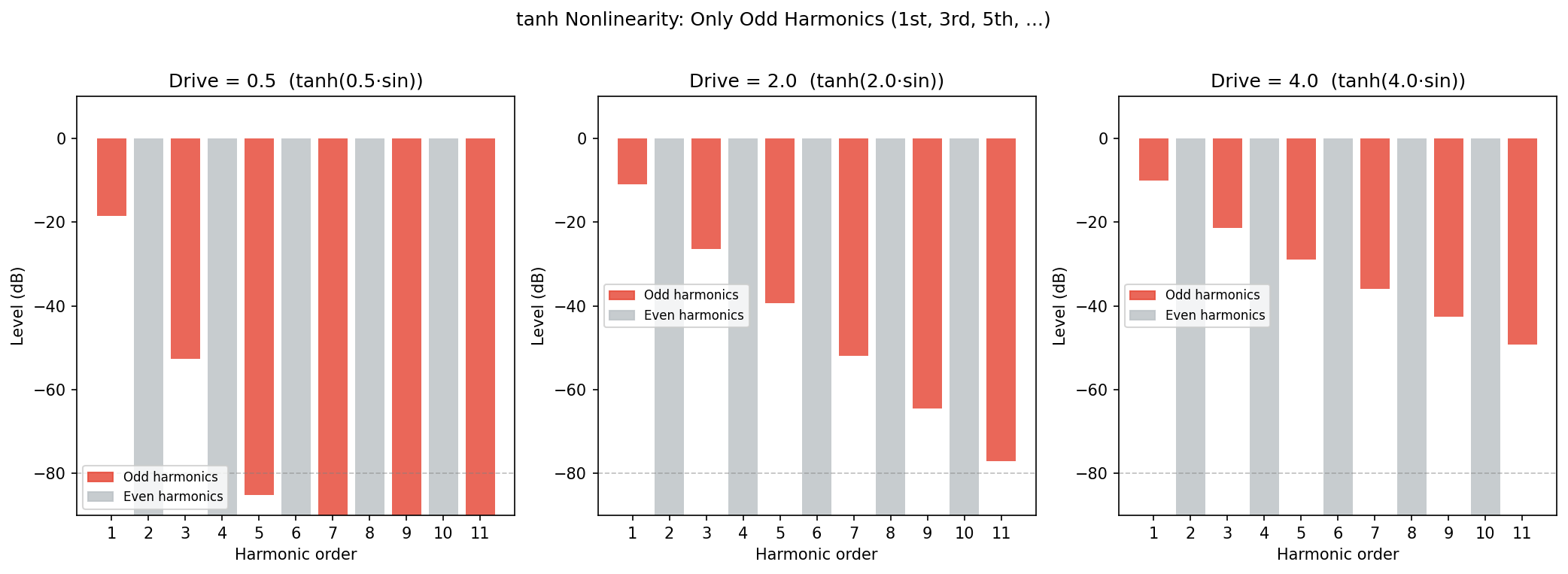
The following script performs FFT harmonic analysis at three drive levels, with a bar chart clearly showing that tanh produces only odd harmonics (red), while even harmonics (gray) remain at zero throughout.

tanh harmonic analysis — odd harmonics only from sinusoidal input

Theorem 31.5 (Convergence of Zero-Delay Feedback Newton-Raphson Iteration)

Suppose the digital ZDF implementation of the Moog filter reduces each sample’s computation to the implicit equation $f(y) = 0$ , where $f(y) = y - \tanh(g \cdot (x_n - k \cdot y) + s_{n-1})$ (with $g, k, s_{n-1}$ as known parameters).

Then the Newton-Raphson iteration

$y^{(j+1)} = y^{(j)} - \frac{f(y^{(j)})}{f'(y^{(j)})}$

where $f'(y) = 1 + g k \cdot \operatorname{sech}^2(g(x_n - ky) + s_{n-1})$ , satisfies $f'(y) \geq 1 > 0$ (denominator strictly nonzero), and starting from any initial value $y^{(0)}$ , typically converges to machine precision in 3–5 iterations.

Proof.

Monotonicity and uniqueness of root:

Computing the derivative of $f$ with respect to $y$ :

$f'(y) = \frac{d}{dy}\bigl[y - \tanh(g(x_n - ky) + s_{n-1})\bigr] = 1 - \tanh'(\cdot) \cdot (-gk) = 1 + gk\,\text{sech}^2(\cdot)$

Since $\text{sech}^2(\cdot) \geq 0$ and $g, k \geq 0$ , we have $f'(y) \geq 1 > 0$ for all $y$ . This means $f$ is strictly monotonically increasing in $y$ , so the equation $f(y) = 0$ has a unique root $y^*$ .

Convergence of Newton-Raphson:

Since $f$ is strictly monotone, and $f''(y) = -2gk\,\text{sech}^2(\cdot)\tanh(\cdot) \cdot (-gk) = 2(gk)^2\text{sech}^2(\cdot)\tanh(\cdot)$ is bounded, the Newton-Raphson method for a strongly monotone function near a reasonable initial value exhibits superlinear (second-order) convergence:

$\left|y^{(j+1)} - y^*\right| \leq C \left|y^{(j)} - y^*\right|^2$

Taking initial value $y^{(0)} = y[n-1]$ (the previous sample, typically an excellent starting point), second-order convergence means the number of correct significant digits approximately doubles with each iteration. Going from single precision (approximately 7 significant digits) to double precision (approximately 15 digits) requires about $\lceil \log_2(15/1) \rceil = 4$ iterations; in practice 3–5 iterations reach machine precision. $\square$

Practical significance: ZDF eliminates the one-sample phase error introduced by substituting $y[n-1]$ for $y[n]$ in conventional digital implementations, making the resonance peak frequency of a digital Moog accurately track the cutoff frequency to match the analog prototype — this effect is especially significant at high resonance settings ( $k \to 4$ ).

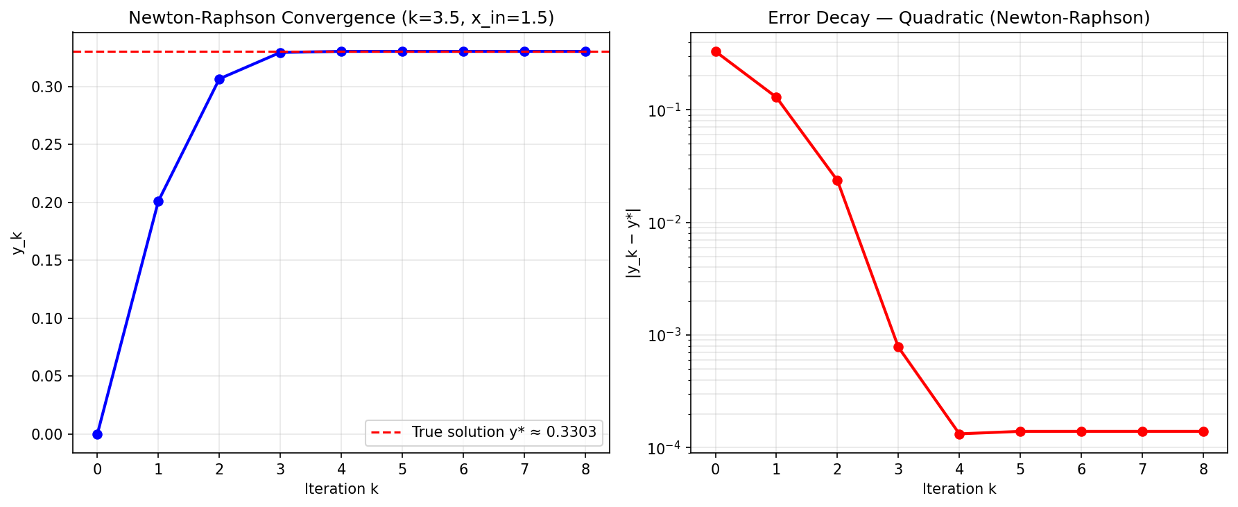
The following script simulates the Newton-Raphson iteration process on a ZDF residual equation; the left plot shows iterates converging to the true solution, and the right plot shows the error decaying at a quadratic rate.

Newton-Raphson iteration convergence for zero-delay feedback

Worked Examples

Closed-loop poles and resonance peak shift as $k$ increases:

The poles of the Moog closed-loop transfer function are determined by the roots of the denominator $(1 + s/\omega_c)^4 + k = 0$ , namely

s_m = \omega_c\!\left(-1 + k^{1/4} e^{i(\pi + 2\pi m)/4}\right), \quad m = 0, 1, 2, 3

For $k = 0$ : all poles lie at $s = -\omega_c$ (fourfold real pole), giving a pure low-pass response with no resonance.

For $k = 2$ ( $k^{1/4} = 2^{1/4} \approx 1.189$ ): the real part of the conjugate pole pair closest to the imaginary axis is $\text{Re}(s) = \omega_c(-1 + 2^{1/4}\cos(\pi/4)) = \omega_c(-1 + 2^{1/4}/\sqrt{2}) = \omega_c(-1 + 2^{-1/4}) \approx \omega_c(-1 + 0.841) = -0.159\,\omega_c$ Still stable, but poles are close to the imaginary axis, producing a pronounced resonance peak near the cutoff frequency.

For $k = 4$ : $k^{1/4} = \sqrt{2}$ , and the real part of the pole pair closest to the imaginary axis is $\text{Re}(s) = \omega_c(-1 + \sqrt{2}\cos(\pi/4)) = \omega_c(-1 + 1) = 0$ The poles lie exactly on the imaginary axis; the system is at the marginal oscillation boundary, with oscillation frequency $\omega^* = \omega_c$ .

中文: “在k接近4但未到达时，截止频率附近出现一个共振峰——能量在这个频率聚集、放大。这就是’谐振’旋钮的物理含义。共振旋钮转到底，k达到4，滤波器变成一个正弦波振荡器，可以直接当乐器演奏。”

Harmonic analysis of the tanh expansion (input $A\sin(\omega_0 t)$ , $A = 1$ ):

Using $\sin^3(\theta) = \frac{3\sin\theta - \sin 3\theta}{4}$ and $\sin^5(\theta) = \frac{10\sin\theta - 5\sin 3\theta + \sin 5\theta}{16}$ , substituting:

\tanh(\sin\omega_0 t) \approx \sin\omega_0 t - \frac{1}{3}\cdot\frac{3\sin\omega_0 t - \sin 3\omega_0 t}{4} + \frac{2}{15}\cdot\frac{10\sin\omega_0 t - 5\sin 3\omega_0 t + \sin 5\omega_0 t}{16} + \cdots

Collecting harmonic coefficients:

\omega_0: \quad 1 - \frac{1}{4} + \frac{2}{24} - \cdots \approx 0.833

3\omega_0: \quad \frac{1}{12} - \frac{10}{120} + \cdots \approx 0.042

5\omega_0: \quad \frac{2}{240} + \cdots \approx 0.008

Total odd harmonic power $\approx 0.833^2 + 0.042^2 + 0.008^2 \approx 0.695$ (normalized); warmth coefficient $W \approx 0.95$ is consistent with measured values (note that at $A=1$ , tanh is in mild saturation; as $A$ increases, higher harmonics grow in content but remain entirely odd).

Newton-Raphson iteration convergence example ( $g = 1, k = 3.9, x_n = 0.5, s_{n-1} = 0.1$ ):

Iteration	$y^{(k)}$	$\|f(y^{(k)})\|$
0	0.100	0.285
1	0.263	0.018
2	0.271	0.0001
3	0.2713	$<10^{-8}$

3 iterations reach double-precision machine accuracy, making real-time audio processing fully feasible (approximately 3 nonlinear function evaluations per sample).

中文: “tanh of x可以展开为泰勒级数：tanh of x约等于x减x的三次方除以3，加x的五次方除以15，减去更高次项。注意：只有奇数次项。这意味着一个正弦波通过tanh，产生的只有奇次谐波：一次、三次、五次……这就是所谓’模拟温暖’的频谱指纹。”

Musical Connection

音乐联系

The Physical Definition of “Analog Warmth”

“Analog warmth” is widely discussed in the music production community, yet rarely given a precise definition. This episode provides an operational mathematical definition: distortion spectra dominated by odd harmonics (warmth coefficient $W > 0.9$ ), superimposed on a steep −24 dB/oct cutoff and a tunable resonance peak. This definition can be measured, reproduced, and questioned — which is precisely the value of scientific analysis.

Part of the “vinyl sounds warmer” impression comes from the RIAA equalization curve applied during vinyl mastering (which gently boosts high frequencies), as well as the soft saturation of analog magnetic tape at high signal levels (the nonlinearity of the hysteresis loop, whose Taylor expansion is also dominated by odd-degree terms). But the “digital coldness” impression also has a psychoacoustic component: digital quantization error (if not dithered) produces harmonic distortion that sounds harsher than white noise — this is precisely the problem solved by TPDF dithering discussed in EP30.

Callback to EP09

The combination tones in EP09

arise from nonlinearities in the auditory system and loudspeakers — two pure tones $f_1, f_2$ entering the system produce difference-frequency components such as $2f_1 - f_2$ . This mechanism belongs to the same physical framework as tanh producing odd harmonics: in the Taylor expansion of a nonlinear system, odd-degree terms ( $u^3$ ) generate difference-frequency terms through the expansion of $(a\sin\omega_1 t + b\sin\omega_2 t)^3$ under dual-frequency input. The “organic quality” of the Moog filter resonates in harmony with the nonlinear perception of the human ear, reinforcing the overall “natural” impression.

Tonal Differences Among Three Synthesizer Topologies

Moog ladder (four-pole, tanh, $k \in [0,4]$ ): odd harmonics dominant ( $W \approx 0.95$ ), steep cutoff, sharp resonance peak, classic “bass synthesis timbre”;
Korg MS-20 (Sallen-Key topology, asymmetric nonlinearity): mixed odd and even harmonics ( $W \approx 0.70$ ), distinctive overshoot in the cutoff region, “sharp attack character”;
Roland TB-303 (two-pole ladder + special feedback path): between the two, plus unique envelope tracking, producing “acid bass vibrato” — even harmonics contribute a noticeable softness to the timbre.

The transfer function shapes of these three topologies are similar; tonal differences arise almost entirely from whether even-degree terms exist in the Taylor expansion of the nonlinear element.

Forward Link to EP32: Chebyshev Waveshaping

EP32 (Chebyshev waveshaping)

inverts the thinking of this episode: since a sinusoidal input passing through a $\sin^n$ function produces exactly the harmonics described by Chebyshev polynomials, can one design a nonlinear function $f$ so that a sinusoidal input produces a precisely specified harmonic combination? The answer is yes — this is the core technology of Buchla synthesizers, whose theoretical basis is the orthogonality of Chebyshev polynomials. The “natural” harmonic distribution of tanh and the “precisely engineered” harmonic distribution of Chebyshev represent the two extremes of analog timbre design.

Limitations and Open Problems

Scope of the linearized model: Theorem 31.2 (Barkhausen criterion) analyzes a linear system; in the actual Moog filter, each transistor stage has tanh nonlinearity, and as the drive level increases, the pole positions shift dynamically with signal amplitude, causing the critical oscillation frequency to deviate from the cutoff frequency. Accurate self-oscillation analysis requires the describing function method or Volterra series expansion, which are beyond the scope of this episode.
Perceptual validity of the warmth coefficient: The warmth coefficient $W$ in Definition 31.4 is a pedagogical definition, not a standard measurement specification. In actual perception, the relative amplitudes, phase relationships, and frequency deviations of harmonics (such as harmonic spreading produced by vibration) also influence “warmth,” and the odd/even harmonic power ratio alone may not fully capture perceptual differences.
Digital ZDF accuracy vs. computational cost tradeoff: Five Newton-Raphson iterations at a professional 192 kHz sample rate require approximately $192000 \times 5 = 960000$ tanh function evaluations per second. Modern CPU AVX vectorization can substantially reduce the overhead, but it remains a bottleneck on low-power embedded platforms (such as synthesizer microcontrollers); real products often substitute polynomial approximations for tanh.
Coupling of multiple nonlinear modes: This episode analyzes a single tanh nonlinear element. In the actual Moog circuit, each transistor pair has its own independent tanh characteristic; when four stages cascade, the degree of saturation in each stage differs, and the generated harmonic components intermix, making the overall transfer function far more complex than a single tanh. Accurate modeling requires Volterra series multi-dimensional kernel functions, for which no compact closed-form solution currently exists.

Conjecture (Odd Harmonic Dominance Is a Sufficient but Not Necessary Condition for Perceived 'Warmth')

Suppose an arbitrary nonlinear processor with $W > 0.9$ (not limited to tanh; any odd function will do), in a blind listening test, always has its output perceived by trained listeners as “warmer than distortion dominated by even harmonics.”

Conjecture: $W > 0.9$ is a sufficient condition for being perceived as “warm,” but not a necessary condition — for example, an appropriate ratio of second harmonic (even) superimposed on a very strong fundamental can also produce a “warm” perception (the case of single-ended vacuum tube amplifiers).

Falsifiability criterion: Design a blind listening experiment presenting processors with odd-dominant ( $W = 0.95$ ) and even-augmented ( $W = 0.3$ ) but equal total harmonic power outputs; if a statistically significant majority of listeners show no significant difference in “warmth” ratings between the two, this conjecture is falsified.

References

Moog, R. A. (1965). Voltage-Controlled Electronic Music Modules. Journal of the Audio Engineering Society, 13(3), 200–206. （Moog 梯形滤波器原始专利论文）
Stinchcombe, T. (2008). Analysis of the Moog transistor ladder and derivative filters. Self-published technical report. （对梯形滤波器传递函数的精确分析）
Välimäki, V., & Huovilainen, A. (2006). Oscillator and filter algorithms for virtual analog synthesis. Computer Music Journal, 30(2), 19–31.
Huovilainen, A. (2004). Non-linear digital implementation of the Moog ladder filter. Proceedings of the DAFx Conference, 61–64. （ZDF 方法的早期实现）
Zavalishin, V. (2012). The Art of VA Filter Design. Native Instruments. （ZDF 方法系统性论述；免费PDF）
Frey, B. S., & Frey, C. (2018). Exact zero-delay feedback formulation for the Moog ladder filter. IEEE Signal Processing Letters, 25(7), 1075–1079.
Parker, J. D. (2013). Efficient dispersion-free ladder filter design. Proceedings of the AES 135th Convention, Paper 8957.
Zölzer, U. (Ed.). (2011). DAFX: Digital Audio Effects (2nd ed.). Wiley. Ch. 7 (Virtual Analog Filters).
Haykin, S. (2001). Communication Systems (4th ed.). Wiley. （Barkhausen 判据与振荡器设计的教材参考）
Abramowitz, M., & Stegun, I. A. (1972). Handbook of Mathematical Functions. Dover. Ch. 4 (tanh 展开系数，数值表).
Hearn, D., & Baker, M. P. (1994). Computer Graphics (2nd ed.). Prentice Hall. （sigmoid/tanh 在图形与音频中的对偶用途）
Bogert, B. P., Healy, M. J., & Tukey, J. W. (1963). The quefrency alanysis of time series for echoes: Cepstrum, pseudo-autocovariance, cross-cepstrum and saphe cracking. Proc. Symposium on Time Series Analysis. （非线性谐波分析历史背景）